
In addition to a few other sources, the major inspiration for this article comes from Wolfgang Beyer: http://www.wolfib.com/Image-Recognition-Intro-Part-1/
Github: https://github.com/wolfib/image-classification-CIFAR10-tf
___________________________________________________________________________
The Challenge of Image Recognition
How can we get computers to simulate visualization and image recognition, when we understand so very little about how it is done with the human mind? Machine learning has given us a good start. The goal of machine learning is to build computing systems that have an ability to perform some task without specifying all of the steps. For example, we've previously shown you how to use machine learning for automated tests to reduce redundant tasks in the already-tight development schedule.
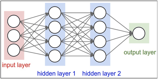
Before we tackle a full-blown solution to computer vision, let’s simplify the task and look at a specific sub-problem. Deep learning recognizes objects in images by using three or more layers of artificial neural networks—in which each layer is responsible for extracting one or more features of the image.

A neural network is a computational model that is analogous to the arrangement of neurons in the human brain. Each neuron takes an input, performs an operation, and then sends output to one or more adjacent neurons. Image recognition is a specific type of object recognition, which is a challenging problem on which conventional neural networks break down.
Image classification and the CIFAR-10 dataset
Here, our aim is to solve a problem that is quite simple, and yet sufficiently challenging to teach us valuable lessons. What we want is for the computer to do this: when it encounters an image having specific image dimensions, the computer should analyze the image and assign a single category to it. This category must be chosen from among a fixed range of various categories. Our goal is construct a model such that it chooses the correct category. This task is known as image classification.
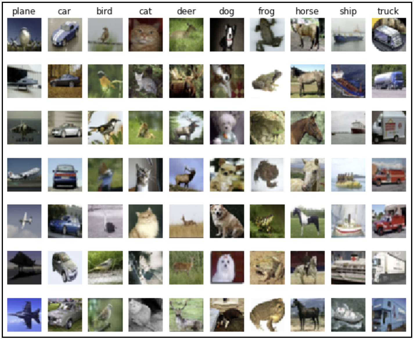
In our tutorial here, we will employ a standardized CIFAR-10 dataset—which contains 60,000 images. In this dataset, there are 10 different categories with 6,000 images in each category. The size of each image is 32 by 32 pixels. Though such a small size often presents a difficulty for a human to identify the correct category, it actually is a simplification for the computer model and reduces the computations necessary to analyze the images.
This figure presents a number of random images from each of the 10 categories in the CIFAR-10 dataset.
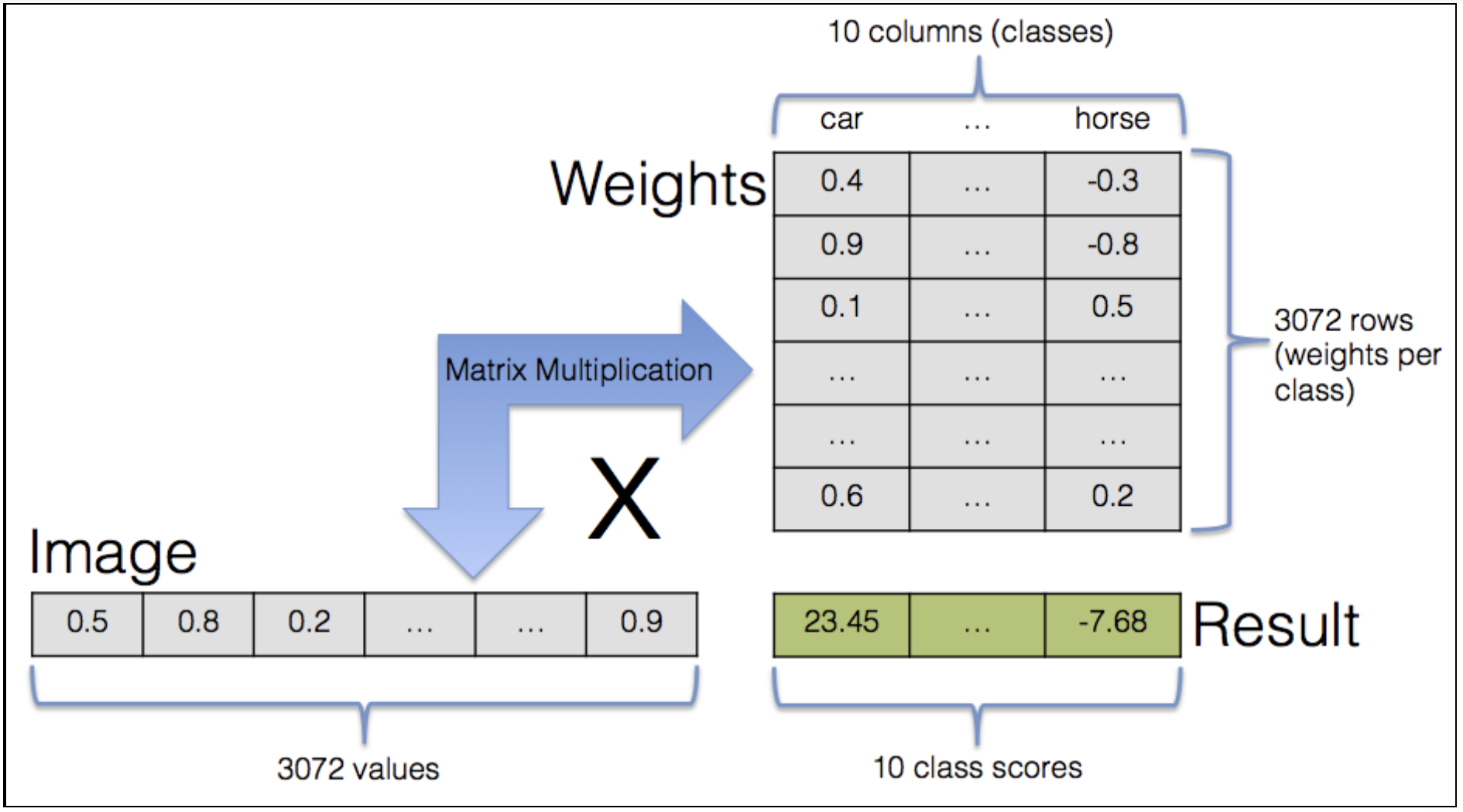
 We can input these images into our model by feeding the model extensive sequences of numbers. Each pixel is identified by three floating-point numbers that represent the red, green and blue values for this pixel (RGB values). This results in a total of 32 x 32 x 3 = 3,072 values for each image.
High quality results are achievable using very large convolutional neural networks. You can learn more on Rodrigo Benenson’s page. Model performance is measured by classification accuracy. Good performance is 90% or above, human performance is an average of 94%, while outstanding results at 96% at best.
Supervised Learning
So, how can we use an image dataset to help a computer “learn”? Even though the computer simulates self-learning, a programmer must first tell it what to learn and how to begin.
It boils down to an optimization problem. We begin with defining the model, and then supply initial values for the model parameters. Then we feed an image dataset into the model, specifying its categories in the model. This is the training stage. During this phase, the model repeatedly examines the training data (from the image dataset), then it iterates while changing the parameter values. The goal is to find those parameter values that result in the model making the highest number of correct identifications. This training is known as supervised learning. Unsupervised learning has the goal of learning from input data that has no labels whatsoever, but that is outside our scope here.
After the training has finished, the model’s parameter values don’t change anymore and the model can be used for classifying images which were not part of its training dataset.
TensorFlow Machine Learning Library
Released by Google in 2015, TensorFlow is a open source software library for machine learning that has quickly become a highly popular machine learning library in use by researchers and other practitioners worldwide. Here, we’ll employ it first for image recognition and then to do the number crunching for our image classification model.
Building the Model, a Softmax Classifier
The remainder of the article presents the work of Wolfgang Beyer, as given in How to Build a Simple Image Recognition System with TensorFlow.
Github: https://github.com/wolfib/image-classification-CIFAR10-tf
The full code for this model is available on Github. To run this code, you’ll first need to install:
- Python — the code has been tested with Python 2.7, but Python 3.3+ should also work
- TensorFlow
- CIFAR-10 dataset — download the Python version of the dataset, or from the compressed archive.
Place the extracted cifar-10-batches-py/ directory into the directory containing the python source code, such that the path to the images will then be:
/[path-to-your-python-source-code-files]/cifar-10-batches-py
Let’s begin by examining the main file of our experiment, softmax.py.
from __future__ import absolute_import
from __future__ import division
from __future__ import print_function
import numpy as np
import tensorflow as tf
import time
import data_helpers
In accordance with the TensorFlow style guide, the future statements should be present in all TensorFlow Python files to ensure compatibility with both Python 2 and 3.
Next, we import TensorFlow, numpy for numerical calculations, the time module, and data_helpers.py which contains functions for loading and preparing the dataset.
beginTime = time.time()
# Parameter definitions
batch_size = 100
learning_rate = 0.005
max_steps = 1000
# Prepare data
data_sets = data_helpers.load_data()
A timer is begun to measure the runtime, then define some parameters—which we detail later. Next is the load of the CIFAR-10 dataset. Since reading the data is not part of the core of what we’re doing, these functions can be found in a separate data_helpers.py file, which reads the dataset files and puts the data into a simple structure.
load_data() will split the 60,000 CIFAR images into two sets: a training set of 50,000 images, and the other 10,000 images go into the test set. When the model parameters can no longer be changed, we’ll input the test set into the model and measure it performance.
Returning to the code, load_data() returns a dictionary containing:
images_train: the training dataset, as an array of 50,000 by 3,072 (= 32 x 32 pixels x 3 color channels) values.labels_train: 50,000 labels for the training set (each a number between 0 and 9 representing which of the 10 classes the training image belongs to)images_test: test set (10,000 by 3,072)labels_test: 10,000 labels for the test setclasses: 10 text labels for translating the numerical class value into a word (such as 0 for ‘plane’, or 1 for ‘car’)
Now we can start building our model. The actual numerical computations are being handled by TensorFlow, which uses a fast and efficient C++ backend to do this. A common workflow is to first define all the calculations we want to perform by building a TensorFlow graph. No calculations are done in this stage, we are only making preparations.
We first describe the type of input data for the TensorFlow graph looks by creating placeholders. These placeholders don’t contain any data, but only specify the type and shape of the input data.
# Define input placeholders
images_placeholder = tf.placeholder(tf.float32, shape=[None, 3072])
labels_placeholder = tf.placeholder(tf.int64, shape=[None])
The placeholders are floating-point values (tf.float32). The shape argument defines the input dimensions. Since we provide multiple images simultaneously, we want to stay flexible about how many images we actually provide. The first dimension of shape is [None], so that the dimension can be of any length. The second dimension is 3,072, which is the number of floating-point values per image.
The placeholder for the class label information contains integer values (tf.int64), in the range from 0 to 9 per image. Since we’re not specifying how many images we’ll input, the shape argument is [None].
# Define variables (these are the values we want to optimize)
weights = tf.Variable(tf.zeros([3072, 10]))
biases = tf.Variable(tf.zeros([10]))
weights and biases are the variables we want to optimize. But let’s talk about our model first.
Our input consists of 3,072 floating point numbers, yet the output we seek is one of 10 different integer values that represents a category. How do we get from 3,072 values to a single one?
The simple approach which we are taking is to look at each pixel individually. For each pixel and each possible category, we want to know whether the color of that pixel increases or decreases the probability that is belongs to a particular category. If, for example the first pixel is red—and If an image of a car often has a first pixel that is red—then we want the score for the car category to increase. We achieve this by multiplying the red color channel value with a positive number and adding that to the car category score.
Similarly, if horse images rarely have a red pixel at position 1, we want that score to decrease. This means multiplying with a small or negative number and adding the result to the horse-score. For each of the 10 categories, we repeat this step on each pixel and then sum up all 3,072 values to get a single overall score. This is a sum of our 3,072 pixel values, weighted by the 3,072 parameter weights for that category. The final result here is that we’ll have 10 scores—one for each category. The highest score gives us our category.
Using matrices, we can greatly simplify the scheme for multiplying the pixel values with weight values and summing up the results. We represent a single image with a 3,072-dimensional vector. If we multiply this vector by a 3,072 x 10 matrix of weights, the result is a 10-dimensional matrix containing exactly the weighted sums we want.
The actual values in the 3,072 x 10 matrix are model parameters. However, if they are random and meaningless then the output will be also. Here we can see the value of the training data, which prepares the model to eventually determine the parameter values by itself.
In the two lines of code above, we inform TensorFlow of the 3,072 x 10 matrix of weighted parameters—all of which have an initial value of 0 in the beginning. We also define a second parameter: a 10-dimensional array containing the bias. The bias does not directly interact with the image data, but is rather added to the weighted sums—a starting point for each scores. Think of an all-black image: all the pixel values are 0, so all of its category scores would be 0 (irrespective of the values in the weights matrix). The biases permit us to begin with non-zero category scores.
The training regimen works like this: First, we input training data and have the model make a prediction using current parameter values. A comparison of that prediction is made with the correct categories, and the numerical result of this comparison is known as loss. The smaller the loss value, the closer the category predictions are to the correct categories—and conversely. The aim is to minimize the loss. But before we look at the loss minimization, let’s take a look at how the loss is calculated.
# Define loss functionloss=tf.reduce_mean(tf.nn.sparse_softmax_cross_entropy_with_logits(logits,labels_placeholder))
TensorFlow handles all the details for us by providing a function which handles all of this. We can then compare the model predictions contained in logits with labels_placeholder, the correct category labels. The output of sparse_softmax_cross_entropy_with_logits() is the loss value for each image. Lastly, we calculate the average loss value across all of the input images.
# Define training operation
train_step = tf.train.GradientDescentOptimizer(learning_rate).minimize(loss)
How do go about varying the parameter values to minimize loss? TensorFlow shines here, using a technique known as auto-differentiation, it calculates the gradient of the loss—with respect to the parameter values. It calculates the influence of each parameter on the overall loss and the extent to which decreasing or increasing it by small amounts would serve to reduce the loss. It seeks to improve accuracy by recursively adjusting all of parameter values. After this step, the process restarts with the next image group.
TensorFlow contains various optimization techniques for translating gradient information into updates for the parameters. For our purpose in this tutorial, we choose the simple gradient descent option, which only examine the current state of the model for determining how to update the parameters and doesn’t consider previous parameter values.
The process for categorizing input images, comparing predictions with the correct categories, calculating loss, and adjusting parameter values is repeated many, many times. Computing duration and cost would quickly escalate with larger and more complex models, but our simple model here doesn’t require much patience or high-performance equipment to see meaningful results.
The next two lines in our code (below) take measures of the accuracy. The argmax of logits along dimension 1 returns the indices of the category with the highest score, which are category label predictions. These labels are compared to the correct category class labels by tf.equal(), which returns a vector of boolean values—which are cast into float values (either to 0 or 1), whose average is the fraction of correctly predicted images.
# Operation comparing prediction with true label
correct_prediction = tf.equal(tf.argmax(logits, 1), labels_placeholder)
# Operation calculating the accuracy of our predictions
accuracy = tf.reduce_mean(tf.cast(correct_prediction, tf.float32))
Now that we have a definition of the TensorFlow graph, we can run it. The graph is accessible in the sess variable (see below). We immediately initialize the variables created earlier. The variable definition initial values are now assigned to the variables.
The iterative training process begins and is repeated max_steps times.
# Run the TensorFlow graph
with tf.Session() as sess:

# Initialize variables
sess.run(tf.initialize_all_variables())
# Repeat max_steps times
for i in range(max_steps):
The next few lines of the code randomly chooses a number of images from the training data:
# Generate batch of input data
indices = np.random.choice(data_sets['images_train'].shape[0], batch_size)
images_batch = data_sets['images_train'][indices]
labels_batch = data_sets['labels_train'][indices]
The first line of code above chooses batch_size random indices between 0 and the size of the training set. Then the batches are built by choosing the images and category labels at these indices.
The resulting groups of images and categories from the training data are known as batches. The batch size indicates how frequently the parameter update step is performed. First, we average the loss over all images in a particular batch, and then update the parameters by means of the gradient descent.
If instead of stopping after a batch and categorizing all images in the training set, we would be able to calculate the true average loss and the true gradient instead of the estimations when working with batches. But it would take a lot more calculations for each parameter update step. At the other extreme, we could set the batch size to 1 and perform a parameter update after every single image. This would result in more frequent updates, but the updates would be a lot more erratic and would quite often not be headed in the right direction. Often, an approach somewhere between those two extremes delivers the quickest improvement of results. It’s often best to pick a batch size that is as large as possible, while still being able to fit all variables and intermediate results into memory.
Every 100 iterations, a check is done on the current accuracy for the training data batch.
# Periodically print out the model's current accuracy
if i % 100 == 0:
 train_accuracy = sess.run(accuracy, feed_dict={
   images_placeholder: images_batch, labels_placeholder: labels_batch})
 print('Step {:5d}: training accuracy {:g}'.format(i, train_accuracy))
Here is the most important line in the training loop, which we model is instructed to perform a single training step:
# Perform the training step
sess.run(train_step, feed_dict={images_placeholder: images_batch,
 labels_placeholder: labels_batch})
All the data has been provided in the TensorFlow graph definition already. TensorFlow knows that the gradient descent update depends the value of the loss, which in turn depends on the logits, which depend on weights, biases, and the actual input batch.
Now it’s necessary only to feed the batch of training data into the model, which is done by providing a feed dictionary—in which the current training data batch is assigned to the placeholders defined above.
After the training is complete, we turn to run the model on the test set. Since this the first time the model encounters the test set, the images are completely new to the model.
The goal, remember, is to assess how adeptly the trained model handles unknown data.
# After finishing the training, evaluate on the test set
test_accuracy = sess.run(accuracy, feed_dict={
 images_placeholder: data_sets['images_test'],
 labels_placeholder: data_sets['labels_test']})
print('Test accuracy {:g}'.format(test_accuracy))
The final lines print how the duration of training and running the model.
endTime = time.time()
print('Total time: {:5.2f}s'.format(endTime - beginTime))
Results
After setting up according to the instructions above and running the model with the command python softmax.py, your output should look something like this:
Step     0: training accuracy 0.14
Step   100: training accuracy 0.32
Step   200: training accuracy 0.3
Step   300: training accuracy 0.23
Step   400: training accuracy 0.26
Step   500: training accuracy 0.31
Step   600: training accuracy 0.44
Step   700: training accuracy 0.33
Step   800: training accuracy 0.23
Step   900: training accuracy 0.31
Test accuracy 0.3066
Total time: 12.42s
The accuracy of evaluating the trained model on the test set is about 31%. If you run the code, you can expect a result in the range of 25-30%. Wolf’s model is able to choose the correct category for an image it first encounters 25% of the time (or better). This is actually fairly impressive.
Since there are 10 different categories, random guessing would result in an accuracy of about 10%. But, if you think that 25% seems quite low, keep in mind that this model is relatively unintelligent. It has no features that would help it discern features such as lines or shapes. It strictly examines the color of each pixel, entirely independent of other pixels. With this in mind, 25% is fair.
More iterations would unlikely improve the accuracy. The results demonstrate that the training accuracy does not steadily increasing, but rather varies between 0.23 and 0.44. It seems that we have found this model limitations, so adding more training data would be unhelpful.
This is a lengthy post, which doesn’t even cover neural nets. But there is an exciting follow-up article available on Wolfgang Beyer’s site that demonstrates how the addition of a small neural network model can significantly improve the results!
If you want to see some image classification in action, you can try out mabl free for three weeks!
___________________________________________________________________________
Sources
http://www.wolfib.com/Image-Recognition-Intro-Part-1/
https://github.com/wolfib/image-classification-CIFAR10-tf
https://www.cs.toronto.edu/~kriz/cifar.html
https://web.stanford.edu/~hastie/CASI_files/DATA/cifar-100.html
https://sourcedexter.com/quickly-setup-tensorflow-image-recognition/
https://www.kernix.com/blog/a-toy-convolutional-neural-network-for-image-classification-with-keras_p14
https://www.learnopencv.com/image-classification-using-convolutional-neural-networks-in-keras/https://machinelearningmastery.com/object-recognition-convolutional-neural-networks-keras-deep-learning-library
https://machinelearningmastery.com/object-recognition-convolutional-neural-networks-keras-deep-learning-library/
http://karpathy.github.io/2011/04/27/manually-classifying-cifar10/
http://rodrigob.github.io/are_we_there_yet/build/classification_datasets_results.html
https://github.com/aleju/imgaug
https://docs.mldb.ai/ipy/notebooks/_tutorials/_latest/Tensorflow%20Image%20Recognition%20Tutorial.html
https://www.tensorflow.org/tutorials/image_recognition
https://hackernoon.com/building-a-facial-recognition-pipeline-with-deep-learning-in-tensorflow-66e7645015b8


